Performance

Description

In this section, the performance of the ppiclF implementation of these algorithms is tested. In the following simulations, ppiclF has been coupled with the incompressible fluid solver Nek5000.

Here, the fluid discritization is composed of hexahedral spectral elements, each with Gauss-Lobatto-Legendre (GLL) quadrature points. Since the GLL points are collocated with the Eulerian field variables, particle-fluid interactions (i.e., Interpolation and Projection) occur between the overlap GLL mesh within each element and nearby particles.

In this example, 9 fields are interpolated and 7 fields are projected, which corresponds to typical multiphase flow simulations. For simplicity, each spectral element is a cube with side lengths \(L_e\) and \(N = 6\) quadrature points in each dimension. Additionally, the entire domain is a cube with side lengths \(L_D\).

Within the domain, \(N_p\) particles are also distributed with uniform random probability in a cube with side lengths of \(L_P\), with this cube being centered inside the GLL elemental domain. Each particle is assumed to be spherical with diameter \(D_p\) and density \(\rho_p\). For projection, a cut-off radius for the Gaussian filter \(r_c/L_e = 0.35\) is used, which bounds the number of grid points each projected particle quantity will be spread over relative to the particle’s coordinates. The soft-sphere collision model in the DEM Packing 3D example is used. In each case, \(L_e = 11.25 \; \text{mm}\), \(\rho_p = 2,500 \; \text{kg/m}^3\), \(k_c = 1,000 \; \text{kg/s}^2\), and \(e_n = 0.9\). Each case was simulated with \(R\) MPI ranks of the Vulcan supercomputer at Lawrence Livermore National Laboratory.

In order to understand how the algorithms in ppiclF perform, we have looked at multiple configurations of the test problem under strong and weak processor scaling. The exact parameters for each case are found in the table below.

Scaling case parameters.

Scaling	Case	\(R\)	\(N_p\)	\(D_p \; (\mu\text{m})\)	\(L_p/L_D \; (\text{m})\)
Strong	1	1,024	25,165,824	511	0.54/0.54
	2	4,096	“	“	“
	3	8,192	“	“	“
	4	16,384	“	“	“
	5	32,768	“	“	“
	6	98,304	“	“	“
Weak	7	1,024	3,145,728	232	0.12/0.54
	8	4,096	12,582,912	“	0.19/0.54
	9	8,192	25,165,824	“	0.24/0.54
	10	16,384	50,331,648	“	0.30/0.54
	11	32,768	100,663,296	“	0.37/0.54
	12	98,304	301,989,888	“	0.54/0.54

Results

For each of these cases, the maximum time on a processor was measured per time step for different algorithms of ppiclF. The strong and weak scaling of these cases in shown in the two figures below on a \(\log_{10}-\log_{10}\) scale. Note that slopes of -1 and -2 are shown in the dashed lines in the strong scaling plot and a slope of 0 is shown on the weak scaling plot.

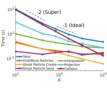
Strong scaling results (cases 1-6).

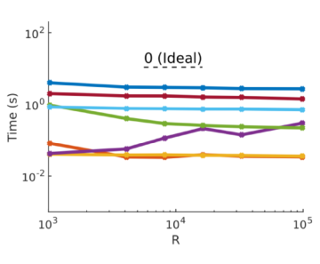
Weak scaling results (cases 7-12).

Additionally, the log-log slopes \(b\) of each of these lines have been computed for a functional scaling of the form \(t = a R^b\) in the table below.

Log-log slopes \(b\) for \(t = a R^b\) for different ppiclF algorithms.

	Strong Scaling	Weak Scaling
Total	-1.36	-0.38
Find/Move	-0.47	-0.15
Ghost Particles	-0.48	0.32
Interpolation	-0.58	-0.64
Projection	-1.03	-0.04
Collision	-1.87	-0.07

In the strong scaling, the problem size is fixed with nearly 25 million particles while the number of processors are increased from approximately \(10^3\) to \(10^5\) ranks. It is observed that collisions dominate the total time taken per time step when \(N_p/R\) is large in case 1. This is expected since the collision algorithm scales as \(O((N_p/R)^2)\) whereas other portions of the algorithm only scale as \(O(N_p/R)\). Despite this, when the number of ranks are increased, the cost of collisions is driven down at a rate of \(R^{-1.87}\) (refer to log-log slope table above) even when \(10^5\) processors are used. Note that -1.87 is close to the algorithmically expected value of -2. Since ideal strong scaling would have a slope of -1, we refer to the collision algorithm as having a “super” scaling. Also, projection and interpolation are the next most costly portions of ppiclF. Projection is more costly than interpolation even though in case 6 they are of comparable cost. Overall, projection has been found to scale as \(R^{-1.03}\) and interpolation as \(R^{-0.58}\). Both projection and interpolation have begun to level off in cases 5-6 even though they perform quite well at first. This is due to the inherent communication associated with the overlap mesh and nearby particles not residing on the same processor. Thus, for greater numbers of particles on a processor (case 1) the communication costs in sending elemental data to the overlapping bins is much less than the computational costs of particle-element interactions. However, when fewer particles per rank are used, the communication costs begin to dominate which is observed in cases 5-6.

In the weak scaling cases, the problem size per processor is fixed at \(N_p/R = 3,072\) as the number of ranks are scaled from approximately \(10^3\) to \(10^5\). This results in over 300 million total particles in case 12. We observe similar trends compared to the strong scaling. Note that an ideal weak scaling slope would be 0 since the problem size per rank doesn’t change. For the most part, the weak scaling of ppiclF is exceptional with most of the algorithmic slopes being less than 0. The reason that most algorithms perform better than ideal is that the bin generation (see Particle Storage) equally partitions the particle domain into a near-ideal distribution with increasing number of processors. The only algorithmic portion which increases under weak scaling is the sending of ghost particles. This routine relies upon the open source GSLIB tool for efficient parallel data transfer under the hood. GSLIB adheres to a logarithmic many-to-many scaling of \(\log_2{R}\) and is the back bone of ppiclF’s parallel communication. Thus, we expect to see this increase in sending ghost particles since the total number of processing ranks is also increasing. While sending ghost particles becomes non-trivial at \(10^5\) processors, if we extrapolate the performance to \(10^6\) ranks we presume that even at such extreme scales ppiclF is not consumed by communication costs.