Particle Storage
Based on the coordinates (\(\mathbf{X}\)) of each individual particle, the particle domain may be decomposed into rectangular prisms in 3D (or simply rectangles in 2D). These rectangular prisms are called bins. The particles with coordinates inside each bin are stored together on the same processor in memory. Additionally, we make the following key assumption: the total number of bins does not exceed the total number of processors.
Bin Generation
In order to decompose the particle domain into bins, a recursive planar cutting is used. Given the bounds of the particle domain, which is the extrema coordinates of all particles in each dimension, the recursive planar cutting algorithm below is used.
c(1:d) = 1
f(1:d) = 0
while Condition 1 and Condition 2 do

   do i=1,d
      c(i) = c(i) + 1

      if Condition 1 or Condition 3 then
         Continue
      else
         c(i) = c(i) - 1
         f(i) = 1
In the previous algorithm, we have defined d to be the number of dimensions (either 2 or 3), c(i) to be a counting array in the i dimension, and f(i) to be a flagging array in the i dimension. The counting array specifies the number of bins in each dimension while the flagging array specifies if more bins can be added in the respective dimension.
Notice that there are three conditions that are checked upon each iteration. The conditions are:
Condition 1 checks the key assumtption: if the total number of bins is less than or equal to the total number of processors.
Condition 2 deals with the size of the bins. Ideally,
c(1)*c(2)*c(3)would be as close to the total number of processors as possible. However, the user may specify a minimum interaction length between nearby particles, calledW. In the current algorithm, this requires the bin lengths in each dimension to be no smaller thanW. Thus, condition 2 checks if the length of the bins in every dimension is the smallest that it can be without being smaller thanW.Condition 3 also deals with the size of the bins. However, condition 3 only checks if the length of the bins in a single
idimension is the smallest that it can be without being smaller thanW.
In 2D, an example of this is shown in the figure below.
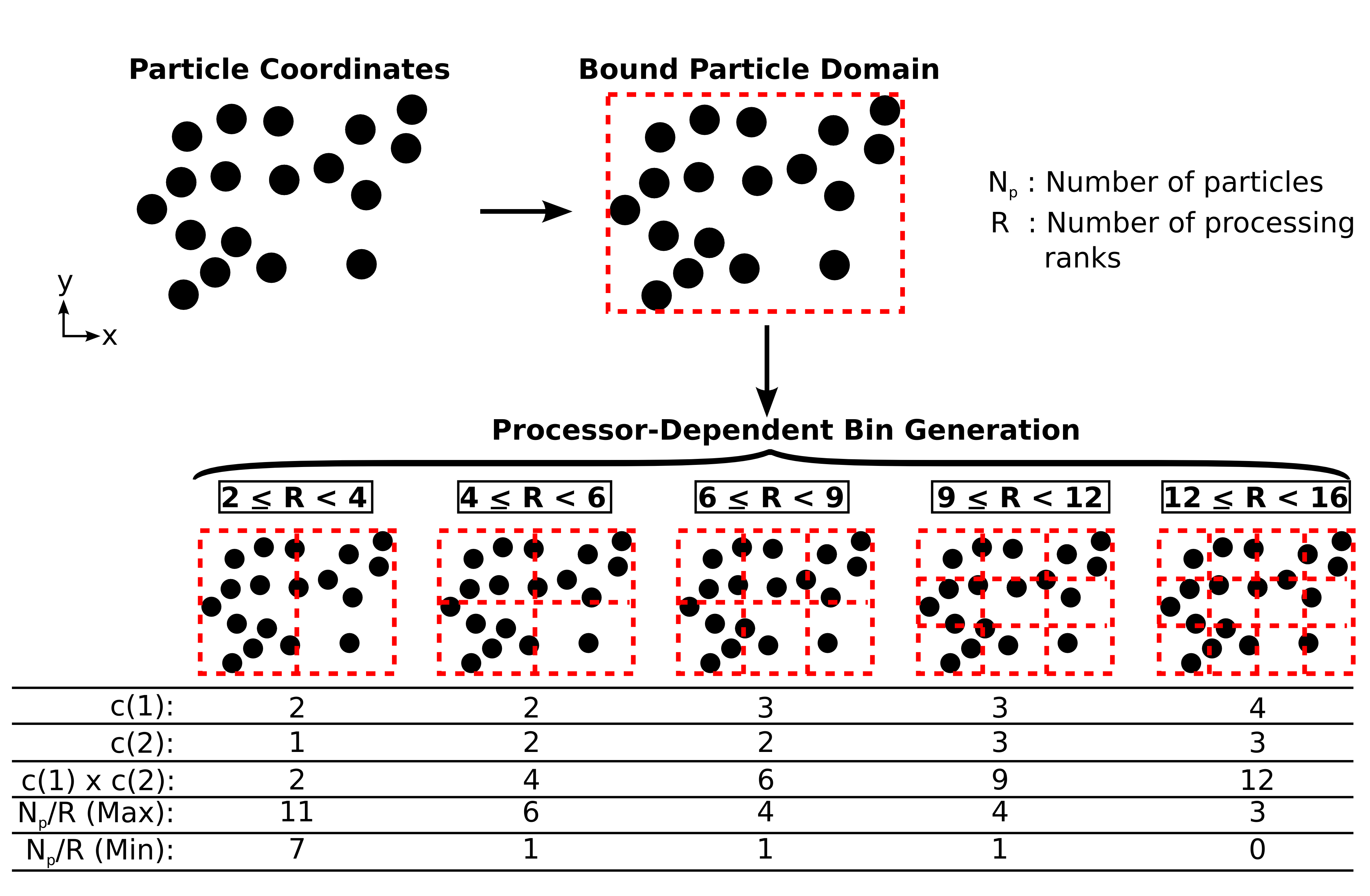
Example of bin generation through recursive planar cutting.
As is shown in the figure, the bin generation begins by bounding the particle domain, which is the region occupied by the rectangular prism whose planes are determined by the global maximum and minimum coordinates of the particles. Following this, the bins, which are demarcated by the dashed lines, are generated through the recursive planar cutting algorithm above. At the end of the process, different bin configurations are realized based on the number of processing ranks used. The resulting bin configurations are shown in the bottom of the figure above.
Additionally, below each bin distribution, the number of particles \(N_p\) per processing rank \(R\) is compared between the different cases. Note that since we have required there to only be one bin stored on each processor, \(N_p/R\) also refers to the number of particles per bin. Ideally, there would be exactly \(N_p/R\) particles on a processor. In the current method, the ideal number of particles per rank is relaxed to allow nearby particles to be locally grouped together in the same rank (or bin). Thus, in the current method we have a deviation from the ideal number of particles on each rank, with ranks having varying numbers of particles. In the figure, the maximum and minimum number of particles on each rank in ppiclF is shown.
Bin-to-Rank Mapping
Once the bins have been created, they are mapped to processing ranks. This includes mapping all the data that has coordinates which are found within the enclosing volume of each bin to the same processor. A single bin is described by the volume which it encloses. To reference a bin, the indices \((i,j,k)\) may be used, where \(i = 0,...,c(1)-1\), \(j = 0,...,c(2)-1\), and \(k = 0,...,c(3)-1\). The volume which each bin encloses is
where \(L_{d*}\) is the particle domain width in respective dimension and \(L_{b*}\) is the bin width in respective dimension (i.e., \(L_{b*} = L_{d*}/c(*)\)).
The bin-to-rank mapping, which determines which processing rank stores the data within a given bin, is then performed by mapping each bins indices \((i,j,k)\) to processing rank \(n_{ID}\) by